Authors:
(1) Maggie D. Bailey, Colorado School of Mines and National Renewable Energy Lab;
(2) Douglas Nychka, Colorado School of Mines;
(3) Manajit Sengupta, National Renewable Energy Lab;
(4) Aron Habte, National Renewable Energy Lab;
(5) Yu Xie, National Renewable Energy Lab;
(6) Soutir Bandyopadhyay, Colorado School of Mines.
Table of Links
Bayesian Hierarchical Model (BHM)
Appendix B: Regridding Coefficient Estimates
4 Solar Radiation Example
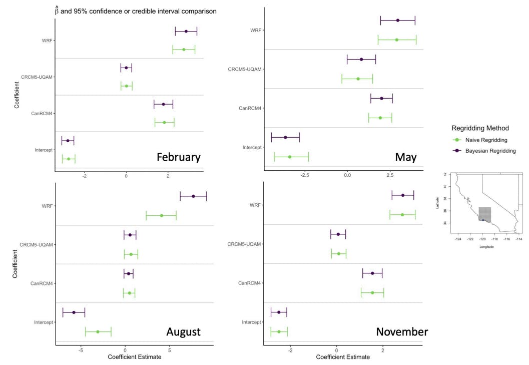
The model described in Sect. 3 was fit once for each location in a subset area of California, shown in the far right bottom panel of Figure 2, which includes coastal and inland areas. Additionally, the model was fit for four separate months (February, May, August, and November) across all years of overlapping data (1998-2009). Initially, all covariates are included in the model. However, not all covariates were found to be significant. In particular, the CanRCM4.ERA-Int was found to hold no significance for the months of February, May, and November for most locations and no significance for about half of the locations in the month of August. The seasonal covariate held no significance for any of the months, which is expected since the data was subset into a single month from each season. Because of this, the seasonal covariate was removed for all four months.
4.1 Posterior Distribution of Model Coefficients
Often, the regridded data set resulting from kriging is used as the ground truth for further analysis. This section outlines the method for analyzing the uncertainty associated with the regridding and linear model prediction step and downstream effects by generating draws from the posterior distributions of each β in Eq. 1.

4.2 Prediction Coverage
This study also considers the coverage of the posterior predictions, i.e. the fraction of days where the prediction interval contains the actual value observed. This portion of the analysis holds out a single year of data as a testing set, using the remaining years as a training set. There are 12 years of overlapping data resulting in 12 out-of-sample prediction results. The final coverage is the average coverage for the 12 folds.
This paper is available on arxiv under CC 4.0 license.

