Authors:
(1) Maggie D. Bailey, Colorado School of Mines and National Renewable Energy Lab;
(2) Douglas Nychka, Colorado School of Mines;
(3) Manajit Sengupta, National Renewable Energy Lab;
(4) Aron Habte, National Renewable Energy Lab;
(5) Yu Xie, National Renewable Energy Lab;
(6) Soutir Bandyopadhyay, Colorado School of Mines.
Table of Links
Bayesian Hierarchical Model (BHM)
Appendix B: Regridding Coefficient Estimates
Appendix A: Simulation Study
Here we implement a short simulation study which highlights some of the main differences, as well as similarities, between the naive method and the BHM.
A1 Simulation Study Setup
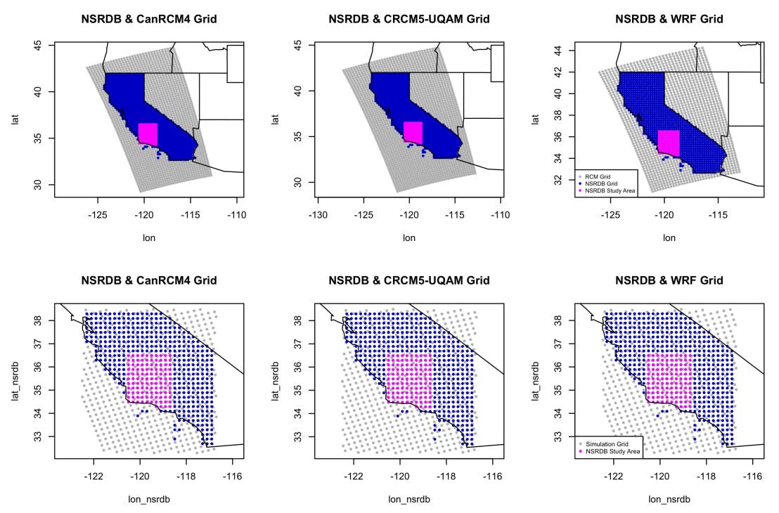
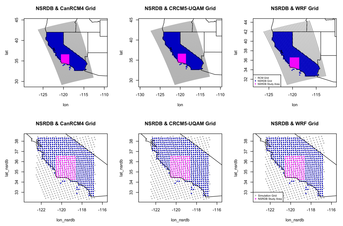
For this simulation study, we utilize the same grids from the original regional climate models. The full grids used in the original study are shown in the top row of Figure A1 with the RCM grids in grey and NSRDB grid over California in blue. The magenta points represent the subsetted area used in the regridding study, which will be also be used in this short simulation study. The bottom row of Figure A1 shows the grids used for this simulation study. The grey and blue dots show the “true" grids which include both the RCM and the NSRDB grid. The magenta points are again the simulation study area on the NSRDB grid. This will be explained more fully in the next section. We added a 2 degree buffer around the final study domain in magenta to avoid any edge effects in the simulation and regridding steps.
A2 Simulation Study Steps
The simulation study follows the steps:
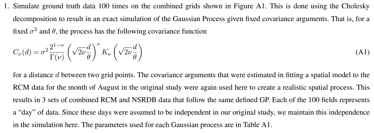
2. Subset the grey points in the bottom row of Figure A1 to only the points that fall on the original RCM grid, in grey in the top row of Figure A1. The “true” NSRDB observations are generated by weighting each RCM grid in a linear model by location:

3. Regridding and model fitting is done for each method in the following way:
(a) Bayesian Regridding: Conditionally simulate each day, or field, 100 times onto the NSRDB Study Area from the RCM grids. For each simulation, run the BHM as described in Section 3.2 and take 50 draws from the posterior distribution for each coefficient resulting in a posterior distribution for each location and for each coefficient.
(b) Naive Regridding: Regrid once from the RCM grid to the NSRDB grid using Kriging. Then estimate a linear model for each location across the 100 days, or fields.
4. Compare the coefficient estimates and standard errors of the coefficients from the naive regridding and the BHM regridding method.
A3 True Coefficients
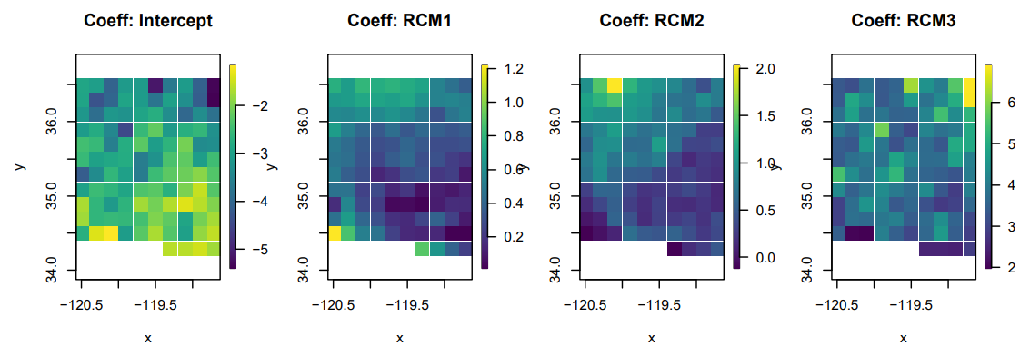
In step 2, the true response, representing the observations from the NSRDB, are generated by weighting each RCM at each location in the study area across all 100 days. These coefficients are set by taking the average βˆ from the BHM in the original manuscript study. The true values for the intercept and each RCM at each location are shown in Figure A2. The weights correspond to the weights estimated for the CanRCM4, CRCM5-UQAM and WRF. The WRF had the highest weight between the three RCMs in the original study.
A4 Results
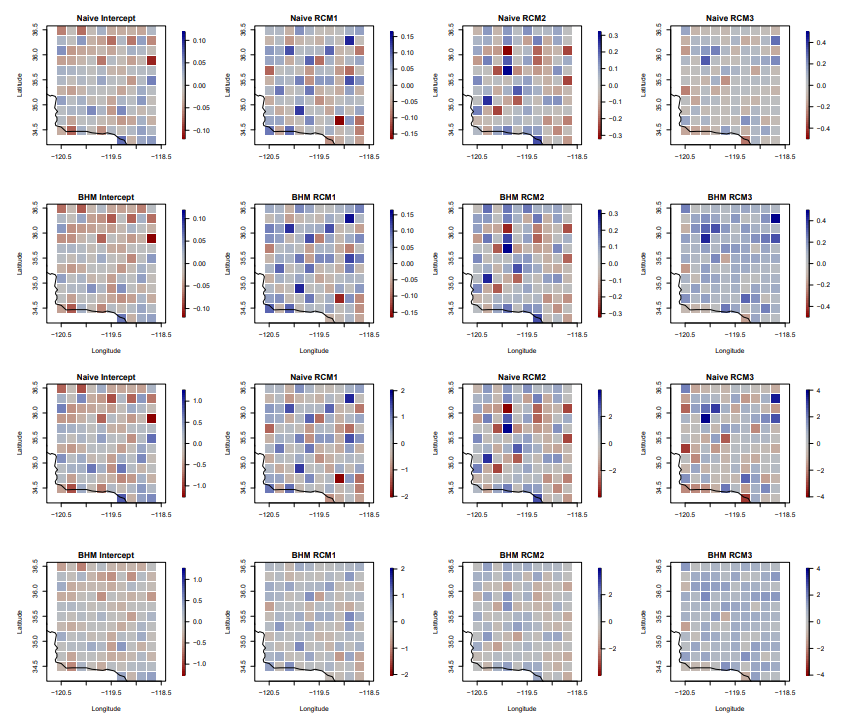
The raw difference relative to the RMSE between the estimated βˆ from the linear model and mean of the posterior distribution for the BHM are shown in Figure A3. Generally, relative to the overall variation of the error, the difference between the true and estimate coefficients is smaller for the BHM and higher for the naive method. This indicates that the regridding uncertainty decreases the raw error in the estimated weights. We also see that for the largest weight (RCM3) the BHM slightly underestimates β3 but the naive method sees larger errors. In general we can say that the bias between the estimates from the BHM is lower than that of the naive regridding method.
We can also look that raw error without normalizing by the RMSE, seen in Figure A3. This figure shows similar errors between the two methods compared to the true coefficients. The exception is seen in the coefficient estimate for RCM3, which is slightly overestimated by the BHM when considering the raw difference compared to the RCM, which slightly underestimates or is closer to the true coefficient.
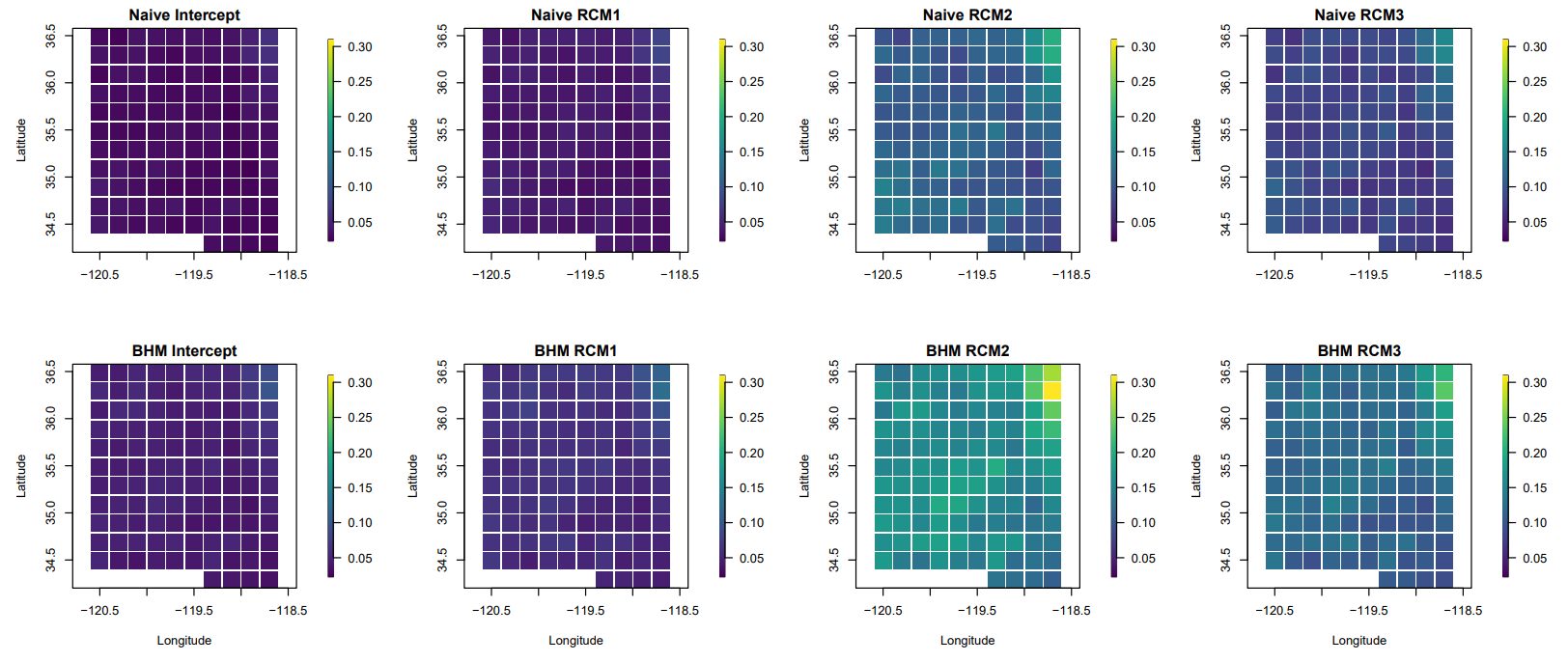
One interesting finding is that the coefficient standard error is larger for the posterior distribution of the BHM estimates than it is for the naive coefficient estimates. This is seen in Figure A4, where the top row shows the standard error for the naive regridding coefficient estimates and the bottom row shows the posterior standard deviations of the BHM estimates. The coefficient standard error for the BHM estimates is on average 46% larger than it is for the naive method. This signifies

that incorporating the regridding uncertainty results in a slightly wider range of potential weights for the RCMs in predicting the observed values. However, the difference in the standard error is not large and because the posterior mean of the BHM coefficient estimates and the naive regridding estimates are very similar, this result may not have much of an effect in this application.
A5 Simulation Study Conclusions
This simulation study highlights some important differences between the naive regridding and BHM regridding methods. In particular, the biases between the true coefficients (weights) and the estimated weights is smaller relative to the error variance for the BHM and larger for the naive method. This indicates that when regridding uncertainty is taken into account, the BHM is more precise in estimating the RCM weights. This finding is further emphasized in the standard error of the coefficients for the two methods. This value is lower for the BHM than it is in the naive method, though the difference in standard error between the two methods is small. Overall we can conclude that taking regridding uncertainty into account results in more precise estimates for model weights when predicting observed values based on climate model output. This precision provides increased understanding in which climate model may have higher importance in predicting observed outcomes and, therefore, future projections for solar radiation.
This paper is available on arxiv under CC 4.0 license.

