A Comprehensive Look at Solar Radiation Predictions through Bayesian Hierarchical Models

Table of Links

Abstract and Intro

Data

Bayesian Hierarchical Model (BHM)

Solar Radiation Example

Results

Conclusion

Appendix A: Simulation Study

Appendix B: Regridding Coefficient Estimates

References

3 Bayesian Hierarchical Model (BHM)

A key part of this study is understanding the predictability of solar radiation based on RCM simulations. Here we organize the statistical assumptions as a BHM for clarity. This helps in tracing the Bayesian approximation used in our application and the standard approach based on regridding also follows as an additional approximation.

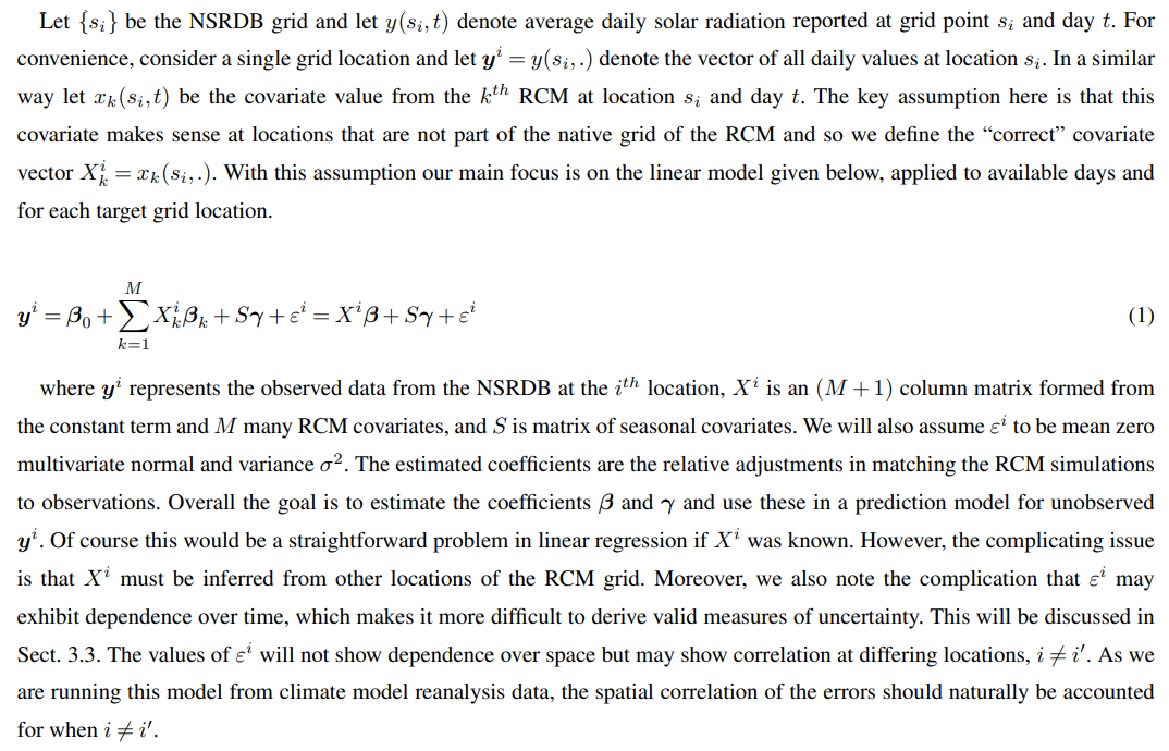
3.1 Observation and Process levels

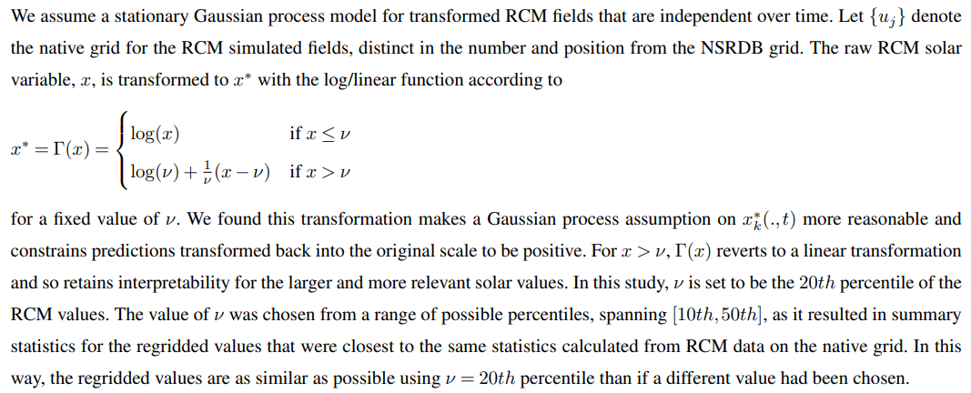
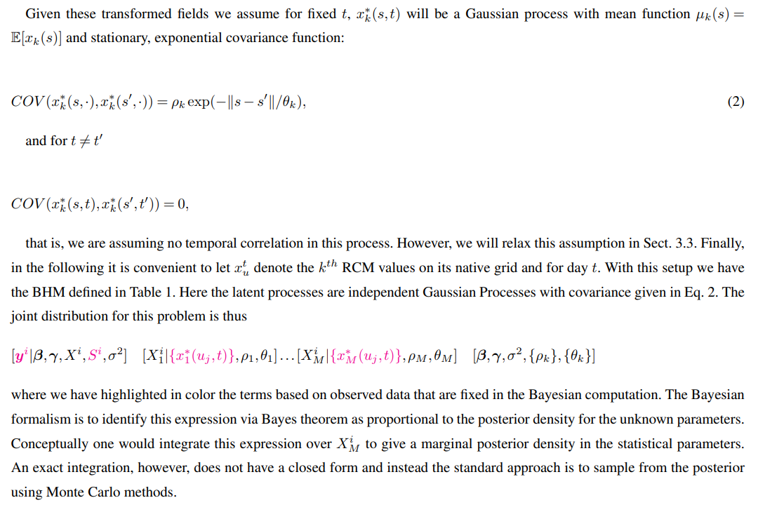
Table 1. BHM for including regridding uncertainty into the coefficient estimates for multi-model analysis.

3.2 Approximate BHM

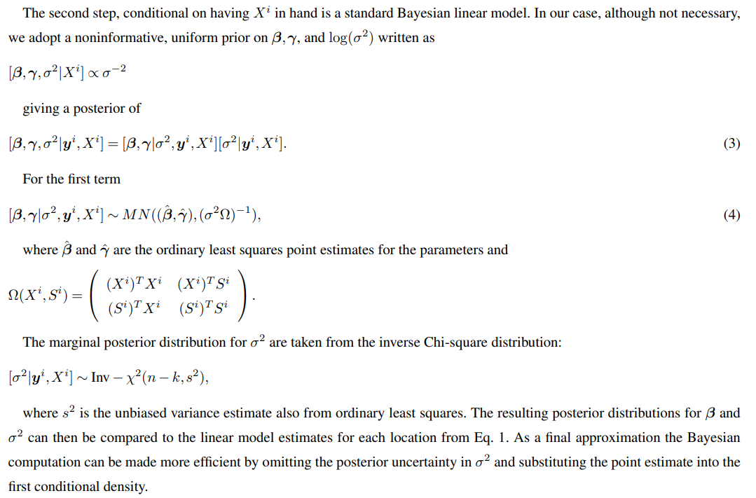
From a Bayesian perspective this posterior is a complete characterization of the uncertainty in all unknown quantities. Unfortunately in this case, as in many BHMs, there is not a closed form for the normalized posterior and so one approximates this distribution. In our case a complete sampling of the posterior is complicated by the fact that the posterior for the Gaussian process covariance parameters is coupled to the linear model through the RCM covariates. Because the linear model only depends on the RCM through its value at the observation grid one can break the sampling into two obvious steps and so doing arrive at the usual strategy used for regridding.

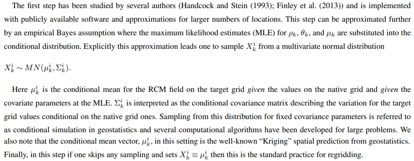
Several regridding methods were considered for this study, including thin plate splines and bilinear interpolation. The chosen method, Kriging with an exponential covariance function, performed the best when considering mean-squared error on test data. Because this study is focused on the uncertainty in this step itself and, more importantly, the downstream effects of the regridding step, a single regridding method was chosen. The differences between regridding and interpolation methods themselves are considered in other studies (McGinnis et al. (2010)).

3.3 Autoreggression Component to BHM

It’s worth mentioning that, in the above analysis, there is no time series addition to explain possible autocorrelation in the residuals. However, we determined a temporal component may not be necessary through fitting several auto regressive moving average models of order p and q (i.e., ARMA(p,q)) and assessing resulting AIC and BIC values. Across the four months considered (February, May, August, November), ARMA(0,0) was largely the best model according to both AIC and BIC. However, in August a MA(2) model had the lowest AIC. Across all months, the model with the second lowest AIC or BIC was frequently a MA(2) or MA(1), followed by an AR(1) model. Although not crucial for our case study for completeness, we have included below how the analysis would change with the addition of a time series component for the Bayesian analysis.

The joint posterior in Eq. 3 becomes

Then, the joint density conditional on all parameters is

and it can be shown that the MA(∞) process has the autocovariance function